spaci

spaci — SPAtial Causal Inference under confounding and interference.

spaci implements two unified methods for estimating the average treatment effect on the treated (ATT) from spatial observational data when spatial confounding (SC) and spatial interference (SI) occur together — a setting where existing methods that address only one of the two are biased:

iDAPS (idaps()) — distance-adjusted propensity score with interference. A matching estimator that matches treated to control units on a data-driven composite of three normalised distances, D = π₁·D^PS + π₂·D^Spatial + π₃·D^Interference. The weights are chosen by minimising a covariate/spatial/exposure balance score, not tuned by hand. Setting π₃ = 0 recovers DAPS and π₂ = π₃ = 0 recovers naive PS.
recoverU+ (recoverUplus()) — a doubly robust estimator whose propensity-score and control-outcome models are augmented with a partially recovered spatial confounder U_R(s) (recovered from the residual Matérn field by GLS) and a neighbourhood-exposure term, so that SC and SI are adjusted for simultaneously.

The naive PS (naive_ps()), DAPS (daps()) and recoverU (recoverU()) comparators, a data simulator (simulate_spatial_causal()) and an all-methods wrapper (spatial_ate()) are also provided.

This package accompanies the report “Unified methods for causal effect estimation: mitigating spatial confounding and interference concomitantly” (Ogunsola, Johnson & House).

Installation

# install.packages("devtools")
devtools::install_github("Ogunsolaia/spaci")

spaci depends only on base R and stats. The recoverU family recovers the spatial confounder via a self-contained Matérn maximum-likelihood fit; to reproduce the report exactly with geoR, install geoR and pass matern_method = "geoR".

Worked example

library(spaci)

## 1. Simulate data with BOTH spatial confounding and interference (true ATT = 2)
sim <- simulate_spatial_causal(n = 250, seed = 1)
##    sim$Y  outcome        sim$X       covariate matrix (X1, X2)
##    sim$Z  0/1 treatment  sim$coords  facility coordinates

## 2. Run every estimator at once (seed fixes the randomised matching order)
res <- spatial_ate(sim$Y, sim$Z, sim$X, sim$coords, tau = 0.1, seed = 1)
res
#>      Method   ATT   SE Lower Upper
#> 1  Naive PS  ...                      <- ignores SC and SI, most biased
#> 2      DAPS  ...
#> 3     iDAPS  ...                      <- adjusts for both
#> 4  recoverU  ...
#> 5 recoverU+  ...                      <- closest to the true ATT

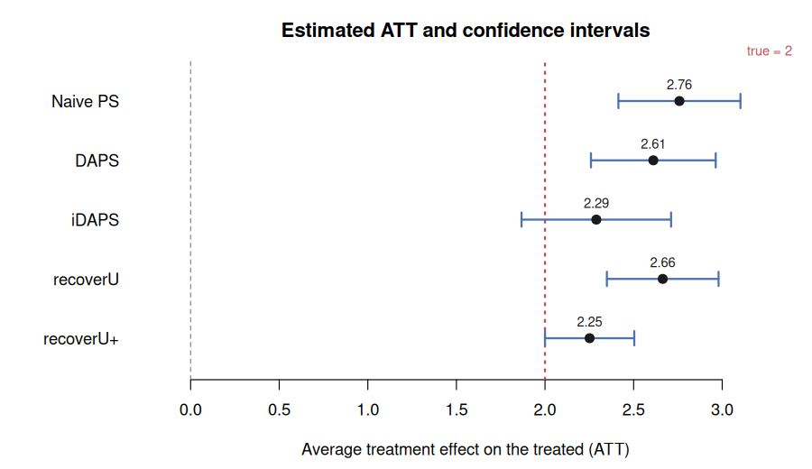
## 3. Visualise the comparison (forest plot, Figure 2.5 style)
plot_ate(res, true_att = sim$true_att)

## 4. Inspect a single method
fit <- idaps(sim$Y, sim$Z, sim$X, sim$coords, tau = 0.1, seed = 1)
fit                     # ATT, CI and the selected (π₁, π₂, π₃) weights
fit$weights             # data-driven composite-distance weights

The forest plot places each method’s ATT and confidence interval against the “no effect” line (0) and the true effect:

On your own data

Supply your outcome, binary treatment, covariates and coordinates directly. The two recommended estimators:

library(spaci)

# Y      numeric outcome            (length n)
# Z      binary treatment 0/1       (length n)
# X      covariates                 (n x p matrix or data frame)
# coords facility/site coordinates  (n x 2 matrix: longitude, latitude)

# iDAPS — matching on the composite distance
idaps(Y, Z, X, coords, tau = 0.1, caliper = 0.25, seed = 1)

# recoverU+ — doubly robust with recovered confounder + interference term
recoverUplus(Y, Z, X, coords, tau = 0.1)

# all five methods side by side, then plot
res <- spatial_ate(Y, Z, X, coords, tau = 0.1, seed = 1)
plot_ate(res)

tau sets the interference kernel bandwidth (smaller = more local); tune it to the spatial scale of your interference.

Inputs

All estimators share the same interface:

Argument	Description
`Y`	numeric outcome vector
`Z`	binary treatment/exposure vector (0/1)
`X`	covariate matrix or data frame
`coords`	two-column matrix/data frame of spatial coordinates
`tau`	spatial decay (bandwidth) of the exposure kernel
`caliper`	maximum matching distance (matching estimators)

Reproducing the simulation study